NumPy 相關功能整理

2023/5/29 程式設計課堂筆記 Python

Array-Oriented Programming with NumPy

介紹
效能比較
建立array
Indexing and Slicing (Getter and Setter)
NumPy calculation methods (Reduction)
- Calculations by Row or Column
array Operators

介紹

Numpy提供了一個高效能的多維度陣列(array)物件
能夠有 array-oriented programming，也就是用函數式的程式設計來處理陣列，讓陣列的操作簡潔而直覺，並且消除了明確編寫迴圈時可能發生的錯誤。

效能比較

NumPy的array和Python的list的差異如下：
- array的大小是固定的，而list的大小是動態的
- array的元素都是同樣的型態，而list的元素可以是不同的型態
- array的運算是向量化的，而list的運算是迭代的
- 在實作上，array是連續的記憶體空間，而list是不連續的記憶體空間
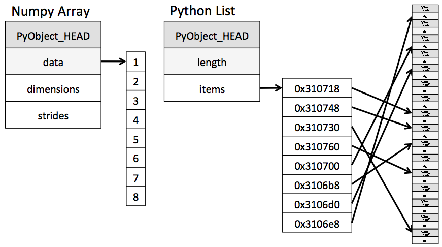
NumPy的array和Python的list的相似點如下：
- array和list都可以儲存多維度的資料

建立`array`

import numpy as np

用`np.array()`建立

numbers = np.array([2, 3, 5, 7, 11])
numbers, type(numbers)
# Output: (array([ 2,  3,  5,  7, 11]), numpy.ndarray)

多維度的`array`

np.array([[1, 2, 3], [4, 5, 6]]), type(np.array([[1, 2, 3], [4, 5, 6]]))
# Output: (array([[1, 2, 3],
#                 [4, 5, 6]]), numpy.ndarray)

`array` Attributes 屬性

屬性	說明
`ndim`	陣列的維度: 一個整數，表示陣列軸的個數，也稱為陣列的階(`rank`)
`shape`	陣列的形狀: 一個由整數組成的元組，表示每個維度中陣列的大小
`size`	陣列的元素個數: `shape`的所有元素相乘
`dtype`	陣列的資料型態
`itemsize`	陣列中每個元素的大小(以位元為單位)

integers = np.array([[1, 2, 3], [4, 5, 6]])
integers.ndim, integers.shape, integers.size
# Output: (2, (2, 3), 6)

floats = np.array([0.0, 0.1, 0.2, 0.3, 0.4])
floats.ndim, floats.shape, floats.size
# Output: (1, (5,), 5)

integers.dtype, floats.dtype
# Output: (dtype('int64'), dtype('float64'))

`array` Methods 方法

方法	說明
`astype()`	轉換陣列的資料型態
`reshape()`	重塑陣列的形狀
`flatten()`	將多維度陣列轉換成一維度陣列
`ravel()`	將多維度陣列轉換成一維度陣列
`dot()`	陣列的內積
`max()`	陣列的最大值
`min()`	陣列的最小值
`mean()`	陣列的平均值
`sum()`	陣列的總和
`std()`	陣列的標準差
`var()`	陣列的變異數
`unique()`	陣列的唯一值
`diagonal()`	陣列的對角線值
`fill()`	陣列的填充值

Creating `array` from sequence generated by different methods

`np.arange()`

和range()類似，參數為numpy.arange(start, stop, step)

np.arange(5)
# Output: array([0, 1, 2, 3, 4])
np.arange(5, 10)
# Output: array([5, 6, 7, 8, 9])
np.arange(10, 1, -2) 
# Output: array([10,  8,  6,  4,  2])

`linspace()`

可以指定要產生的數列的個數，參數為numpy.linspace(start, stop, num)

np.linspace(0.0, 1.0, num=5)
# Output: array([0.  , 0.25, 0.5 , 0.75, 1.  ])

Reshaping an `array`

np.arange(1, 21).reshape(4, 5)
# Output: array([[ 1,  2,  3,  4,  5],
#                [ 6,  7,  8,  9, 10],
#                [11, 12, 13, 14, 15],
#                [16, 17, 18, 19, 20]])

`List` vs. `array` Performance: Introducing `%timeit`

import random
%timeit rolls_list = [random.randint(1, 6) for i in range(0, 6_000_000)] #_ is use to separate long integer
%timeit rolls_array = np.random.randint(1, 7, 6_000_000)

Indexing and Slicing (Getter and Setter)

grades = np.array([[87, 96, 70], [100, 87, 90],
                   [94, 77, 90], [100, 81, 82]])
grades
# Output: array([[ 87,  96,  70],
#                [100,  87,  90],
#                [ 94,  77,  90],
#                [100,  81,  82]])

一維度陣列的索引和切片

grades[0]
# Output: array([87, 96, 70])

多維度陣列的索引和切片

grades[1, 0]
# Output: 100

grades[0:2]
# Output: array([[ 87,  96,  70],
#                [100,  87,  90]])

grades[[1, 3]]
# Output: array([[100,  87,  90],
#                [100,  81,  82]])

grades[:, 0]
# Output: array([ 87, 100,  94, 100])

grades[:, 1:3]
# Output: array([[96, 70],
#                [87, 90],
#                [77, 90],
#                [81, 82]])

Views: Shallow Copies

numbers = np.arange(1, 6)
numbers2 = numbers.view()
id(numbers), id(numbers2)
# Output: (140539985316368, 140539985316928), We can see that the two arrays have different memory addresses
np.shares_memory(numbers, numbers2)
# Output: True, We can see that the two arrays share the same memory
# To prove that `numbers2` views the same data as `numbers`, let's modify an element in `numbers`, then display both arrays:
numbers[1] *= 10
numbers2
# Output: array([ 1, 20,  3,  4,  5])
# Similarly, changing a value in the view also changes that value in the original array:
numbers2[1] /= 5
numbers, numbers2
# Output: (array([ 1,  4,  3,  4,  5]), array([1, 4, 3, 4, 5]))

Copies: Deep Copies

numbers = np.arange(1, 6)
numbers2 = numbers.copy()
id(numbers), id(numbers2)
# Output: (140539985316368, 140539985316928), We can see that the two arrays have different memory addresses
np.shares_memory(numbers, numbers2)
# Output: False, We can see that the two arrays do not share the same memory
# To prove that `numbers2` copies the same data as `numbers`, let's modify an element in `numbers`, then display both arrays:
numbers[1] *= 10
numbers
# Output: array([ 1, 40,  3,  4,  5])
numbers2
# Output: array([1, 2, 3, 4, 5])

Note: Recall that if you need deep copies of other types of Python objects, pass them to the copy module’s deepcopy() function.

More about Reshaping and Transposing

reshape() 和 resize() 都可以改變陣列的形狀，但是 reshape() 只是回傳一個新的陣列，而 resize() 則是直接改變原本的陣列。

grades = np.array([[87, 96, 70], [100, 87, 90]])
grades
# Output: array([[ 87,  96,  70],
#                [100,  87,  90]])
grades.reshape(1, 6)
grades2[0, 0] = 0
grades2, grades
# Output: (array([[ 0, 96, 70, 100, 87, 90]]), array([[ 0, 96, 70],
#                                                  [100, 87, 90]]))

一個常用的技巧是使用 -1 來代表剩下的維度，例如 grades.reshape(-1) 會回傳一個一維度的陣列。

grades.reshape(-1)
# Output: array([ 0, 96, 70, 100, 87, 90])

Note: The reshape() method returns a view if the new shape is compatible with the original shape. Otherwise, it returns a copy.
resize會直接改變原本的陣列

grades.resize(1, 6)
grades
# Output: array([[ 0, 96, 70, 100, 87, 90]])

flatten() and ravel()

flattened = grades.flatten()
flattened
# Output: array([ 0, 96, 70, 100, 87, 90])
flattened[0] = 100
flattened, grades
# Output: (array([100,  96,  70, 100,  87,  90]), array([[ 0, 96, 70],
#                                                      [100, 87, 90]]))
raveled = grades.ravel()
raveled
# Output: array([ 0, 96, 70, 100, 87, 90])
raveled[0] = 100
raveled, grades
# Output: (array([100,  96,  70, 100,  87,  90]), array([[100,  96,  70],
#                                                      [100,  87,  90]]))

Transposing Rows and Columns

transpose = grades.T
transpose
# Output: array([[100, 100],
#                [ 96,  87],
#                [ 70,  90]])

Note: The T attribute returns a view of the array. It does not return a copy.

Stacking

grades2 = np.array([[94, 77, 90], [100, 81, 82]])

np.hstack((grades, grades2))
# Output: array([[ 0, 96, 70, 94, 77, 90],
#                [100, 87, 90, 100, 81, 82]])
np.vstack((grades, grades2))
# Output: array([[ 0, 96, 70],
#                [100, 87, 90],
#                [ 94, 77, 90],
#                [100, 81, 82]])

`NumPy` calculation methods (Reduction)

一個陣列包含了許多方法可以計算陣列中的元素，預設上這些方法會忽略陣列的形狀，並且使用所有的元素來計算。例如計算平均值時，會將所有的元素加總後除以總數。我們也可以針對每個維度來執行這些計算，例如在二維陣列中，我們可以計算每一列和每一行的平均值。

grades = np.array([[87, 96, 70], [100, 87, 90],
                   [94, 77, 90], [100, 81, 82]])
grades
# Output: array([[ 87,  96,  70],
#                [100,  87,  90],
#                [ 94,  77,  90],
#                [100,  81,  82]])
print(grades.sum())
print(grades.min())
print(grades.max())
print(grades.mean())
print(grades.std())
print(grades.var())
# Output: 1054
#         70
#         100
#         87.83333333333333
#         8.781612133840075
#         77.30555555555556

Calculations by Row or Column

數值計算方法可以針對特定的維度來計算，這個維度被稱為 axis。這些方法可以接受一個 axis 參數來指定要使用的維度，這個參數提供了一個方便的方法來在二維陣列中針對每一列或每一行來計算。

# 假設我們想要找到每一次考試的最高分數，以列來說就是每一次考試的最高分數，以行來說就是每一個學生的最高分數。
# 這個計算可以使用 `axis` 參數來指定要使用的維度，`axis=0` 代表要針對每一列來計算，`axis=1` 代表要針對每一行來計算。
grades, grades.max(axis=0), grades.argmax(axis=0)
# Output: (array([[ 87,  96,  70],
#                 [100,  87,  90],
#                 [ 94,  77,  90],
#                 [100,  81,  82]]), array([100,  96,  90]), array([1, 0, 1]))
grades, grades.mean(axis=0)
# Output: (array([[ 87,  96,  70],
#                 [100,  87,  90],
#                 [ 94,  77,  90],
#                 [100,  81,  82]]), array([95.25, 85.25, 83.  ]))
# 因此，95.25 代表第一列的平均值 (87, 100, 94, 100)，85.25 代表第二列的平均值 (96, 87, 77, 81)，83 代表第三列的平均值 (70, 90, 90, 82)。
# 同樣的，指定 `axis=1` 會針對每一行的所有列來計算。要計算每一個學生的平均分數，我們可以使用：
grades, grades.mean(axis=1)
# Output: (array([[ 87,  96,  70],
#                 [100,  87,  90],
#                 [ 94,  77,  90],
#                 [100,  81,  82]]), array([84.33333333, 92.33333333, 87.        , 87.66666667]))

`array` Operators

The slowness of loops

計算 NumPy 陣列的速度可以從非常快到非常慢，為了優化效能，建議使用向量化的操作，這些操作通常是透過 NumPy 的通用函式 (ufuncs) 來實作。在執行許多小操作的情境中，Python 的運算速度通常會變得明顯的緩慢。其中一個例子是當我們使用迴圈來對陣列中的每個元素執行操作。例如，假設我們有一個值的陣列，並且需要計算每個值的倒數。一個直接的方法可能會包含：

def compute_reciprocals(values):
    output = np.empty(len(values))
    for i in range(len(values)):
        output[i] = 1.0 / values[i]
    return output

values = np.random.randint(1, 10, 5)
compute_reciprocals(values)
# Output: array([0.5       , 0.33333333, 0.5       , 0.5       , 0.25      ])

但是如果我們測量這段程式碼的執行時間，我們會發現這段程式碼的執行速度非常慢：

big_array = np.random.randint(1, 10, 1_000_000)
%timeit compute_reciprocals(big_array)
# Output: 1.55 s ± 9.21 ms per loop (mean ± std. dev. of 7 runs, 1 loop each)

Element-wise arithmetic

NumPy提供了許多運算子，讓我們可以建立簡單的運算式，這些運算式可以對整個陣列進行操作，並返回另一個陣列。首先，讓我們使用算術運算子和擴增指定來執行陣列和數值之間的元素運算。元素運算是針對每個元素進行的，因此下面的片段會將每個元素加倍並將每個元素立方。每個運算都會返回一個包含結果的新陣列：

numbers = np.arange(1, 7) # array([1, 2, 3, 4, 5, 6])
numbers * 2
# Output: array([ 2,  4,  6,  8, 10, 12])
numbers ** 3
# Output: array([  1,   8,  27,  64, 125, 216])

增廣指定運算子也可以用來修改現有陣列的值。

numbers += 10
numbers
# Output: array([11, 12, 13, 14, 15, 16])

Broadcasting

典型地，算術運算需要兩個與操作數相同大小和形狀的陣列。當一個操作數是單個值時，稱為標量，NumPy會像樣的陣列一樣進行元素運算，但是標量值存在於所有元素中。這被稱為廣播。上面的片段演示了這種能力。例如，numbers * 2 等同於 numbers * [2, 2, 2, 2, 2, 2]。

Arithmetic Operations Between `arrays`

numbers2 = np.linspace(1.1, 6.6, 6) # 算術運算子可以用於兩個陣列，並且會對相應的元素進行運算。
numbers * numbers2 # array([11, 12, 13, 14, 15, 16]) * array([ 1.1,  2.2,  3.3,  4.4,  5.5, 6.6])
# Output: array([12.1, 26.4, 42.9, 61.6, 82.5, 105.6])
c = np.ones((3, 3)) # 算數運算子也可以用在整數和浮點數陣列之間。
c * c 
# Output: array([[1., 1., 1.],
#                [1., 1., 1.],
#                [1., 1., 1.]])
# 進行矩陣乘法，可以使用 dot 函式或 @ 運算子。
1. c.dot(c) 
2. c @ c 
  # Output: array([[3., 3., 3.],
  #                [3., 3., 3.],
  #                [3., 3., 3.]])
# 我們可以把廣播應用到更高維度的陣列，例如，考慮將一維陣列加到二維陣列，並觀察結果：
a = np.array([0, 1, 2])
M = np.ones((3, 3))
print(a.shape, M.shape)
M + a
# Output: array([[1., 2., 3.],
#                [1., 2., 3.],
#                [1., 2., 3.]])
# 在這裡，一維陣列 a 被拉伸或廣播，以匹配 M 的形狀。

Rules of Broadcasting

在 NumPy 中，廣播遵循一套嚴格的規則，這些規則規定了兩個陣列如何相互交互。這些規則如下：

當兩個陣列之間的維度數量不同時，陣列的維度較少的一方在其前面（左側）填充一個維度，以匹配另一個陣列的維度數量。
如果兩個陣列在任何維度上的形狀都不匹配，則在該維度上形狀為 1 的陣列會擴展以匹配另一個陣列的形狀。
如果兩個陣列在任何維度上的大小衝突，並且都不等於 1，則會引發錯誤。

看一個例子：

a = np.arange(0, 40, 10).reshape(4,1)
b = np.arange(3)
print(a.shape, b.shape)
a + b
# Output: array([[ 0,  1,  2],
#                [10, 11, 12],
#                [20, 21, 22],
#                [30, 31, 32]])

要開始，我們需要確定兩個陣列的形狀：a.shape 是 (4,1)，b.shape 是 (3,)。根據規則 1，我們必須在 b 的形狀中添加 1，以使其維度與 a 的維度匹配。因此，b.shape 變成 (1,3)。
接下來，規則 2 規定，我們需要擴展 b.shape 中的每個 1，以匹配另一個陣列的相應大小。因此，a.shape 變成 (4,3)，而 b.shape 變成 (4,3)，因為 1 被複製了三次以匹配 a 的大小。
由於兩個陣列的形狀現在匹配，因此它們是兼容的。

這整個過程可以如下圖所示：

Comparing arrays

numbers >= 13 # numbers = array([11, 12, 13, 14, 15, 16])
# Output: array([False, False, True, True, True, True])
numbers2 < numbers # numbers2 = array([ 1.1,  2.2,  3.3,  4.4,  5.5, 6.6])
# Output: array([ True,  True,  True,  True,  True,  True])
numbers == numbers2
# Output: array([False, False, False, False, False, False])
numbers == numbers
# Output: array([ True,  True,  True,  True,  True,  True])

Universal Functions (Vectorization)

現在我們將深入研究 NumPy 如何在不使用 for 迴圈的情況下對 array 執行元素級操作：

NumPy 提供了更多的運算子/函式作為獨立的通用函式（也稱為 ufuncs），這些函式以元素級的方式執行各種操作，這意味著它們將相同的操作應用於 array 中的每個元素。
- 這些函式對一個或兩個類似 array 的參數（例如 lists）進行操作，並用於執行任務。
- 當使用 array 與 + 和 * 等運算子時，會自動調用其中一些函式。每個 ufunc 生成一個新的 array，其中包含操作的結果。
NumPy 提供一個實用的接口，用於各種直接訪問靜態類型和編譯過程的操作。
- 這些操作稱為向量化操作。通過使用 array 操作（例如加法、減法、乘法和除法），可以實現向量化。
- 此外，還可以通過使用 ufunc 來實現。這些向量化方法旨在將循環移動到支撐 NumPy 的編譯層，從而讓執行速度更快。

Exploring `NumPy`’s `Ufuncs`

把兩個 array 相加，NumPy 會自動調用 add() 函式：

numbers2 = np.arange(1, 7) * 10  # array([10, 20, 30, 40, 50, 60])
np.add(numbers, numbers2)        # equivalent to numbers + numbers2, numbers = array([11, 12, 13, 14, 15, 16])
# Output: array([21, 32, 43, 54, 65, 76])

Broadcasting with Universal Functions

使用 multiply() 通用函式將 numbers2 的每個元素乘以標量值 5：

np.multiply(numbers2, 5) # equivalent to numbers2 * 5
# Output: array([ 50, 100, 150, 200, 250, 300])

# 重塑 numbers2 成為一個 2x3 的陣列，然後將其值乘以一維陣列的三個元素：
numbers3 = numbers2.reshape(2, 3)
numbers4 = np.array([2, 4, 6])
numbers3, numbers4
# Output: (array([[10, 20, 30],
#                 [40, 50, 60]]),
#          array([2, 4, 6]))
np.multiply(numbers3, numbers4) # Equivalent to numbers3 * numbers4
# Output: array([[ 20,  80, 180],
#                [ 80, 200, 360]])

在這種情況下，numbers4 的長度與 numbers3 的每一行相同，允許 NumPy 將乘法操作應用於 array，並將 numbers4 視為具有以下值的 array：

array([[2, 4, 6],
       [2, 4, 6]])

如果通用函式接收到兩個不支持廣播的不同形狀的 array，則會引發 ValueError。
向量化和 ufunc 函式與 NumPy 中的廣播緊密相關，因為它們經常一起使用，以在具有不同形狀的 array 上執行元素級操作。
通過結合向量化、ufunc 函式和廣播，我們可以有效地在 NumPy array 上執行複雜的算術操作。

還有其他特殊的數學 ufunc。讓我們創建一個陣列，並使用 sin() 通用函式計算其值的平方根：

numbers = np.array([1, 4, 9, 16, 25, 36])
np.sin(numbers)
# Output: array([ 0.84147098, -0.7568025 ,  0.41211849, -0.28790332, -0.13235175, -0.99177885])

Create our own vectorizing functions

向量化操作通常更簡潔，因此建議避免對向量和矩陣進行逐元素循環，而是使用向量化算法。
將標量算法轉換為向量化算法的初始步驟涉及驗證我們創建的函式是否可以使用向量輸入運行：

def Theta(x, th):
    """
    Scalar implemenation of a variant of Heaviside step function.
    """
    if x >= th:
        return 1
    else:
        return 0

Theta_vec = np.vectorize(Theta)
Theta_vec(np.array([-3,-2,-1,0,1,2,3]), 1)
# Output: array([0, 0, 0, 0, 1, 1, 1])

LOADING